
Task solution - fast Fourier transform in fortran (using fftw3)
This repository contains the realization of the second task of the fortran programming language course at AGH in Cracov.
Directory structure
Makefile
README.md
src/
    fourier.F90
    f1_dft.gnuplot
    f1_original.gnuplot
    f2_dft.gnuplot
    f2_filtered.gnuplot
    f2_original.gnuplot
res/
    f1_dft.txt
    f1_original.txt
    f2_dft.txt
    f2_filtered.txt
    f2_original.txt
    f1_dft.png
    f1_original.png
    f2_dft.png
    f2_filtered.png
    f2_original.png
Makefile
This file contains recipes for building the fortran program and using to generate plots.
src/
This directory contains the fortran source of the project, namely fourier.f90 and gnuplot scripts for generating png plots.
res/
This directory contains relevant plots of signals and frequency spectrums as required for the task.
Building
As a prerequisite, fftw3, make and a fortran compiler, either gfortran or ifort, are required (didn't want to support proprietary compiler :c but had to). It is assumed, that include files for fftw3 are installed under /usr/include.
Run
$ make
to build the program executable fourier.
The makefile checks which one of the 2 compilers is present and uses it. Alternatively, one can specify fortran compiler explicitly, e.g.
$ make FC=gfortran
or
$ make FC=ifort
Running
The executable is fourier. It's mandatory first argument is name of the function to work with - 'f1' or 'f2'. If there're no other arguments - program prints datapoints for plotting the original function. If second argument is 'dft' - program prints datapoints of function's frequency spectrum as obtained from discrete fourier transform. If second argument is 'filtered' - program prints datapoints of filtered function (with frequency components of low values removed).
 $ ./fourier f2 filtered
 0.0000000000000000         0.99737967443382569
 1.5259021896696422E-005    0.99737363952277114
 3.0518043793392844E-005    0.99736759544407216
 4.5777065690089265E-005    0.99736154219778428
 ⋮
 0.99996948195620661         0.99739772416056849
 0.99998474097810330         0.99739171675277982
 1.0000000000000000         0.99738570017718042
Text files and plots in res/ can be regenerated by issuing
$ make pngs
from the main project directory.
Fast Fourier transform
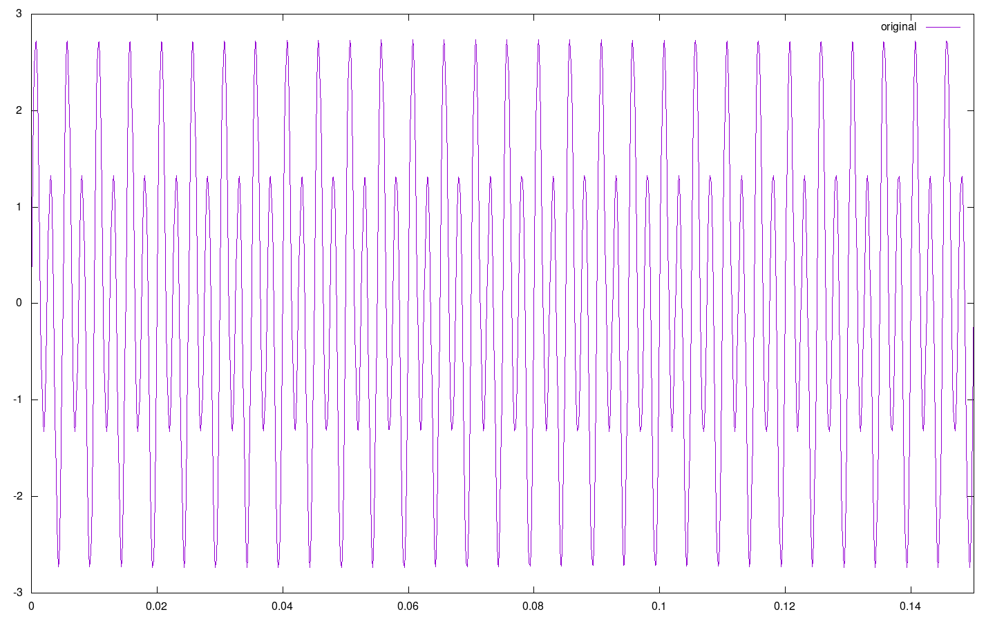
The first part of the task was to use fftw3 library to convert the signal x = sin(2·π·t·200) + 2·sin(2·π·t·400) (represented by function f1 in the program) into sum of signals. To perform the discrete Fourier transform, I took values of f1() at 8192 equadistant points from 0.0 to 1.0. The plot of this function (with x axis constrained to [0.0; 0.15] so that anything can be seen) is
 In general, the result of a Fourier transform is the frequency spectrum of the input signal. In case of dft we don't get a continuous spectrum, but rather a sequence of values representing the strength of their respective frequency components in the signal. Those values can be plotted and connected by lines to get an approximation of the continuous spectrum. Te result of doing this for f1 (y scale logarithmic) is
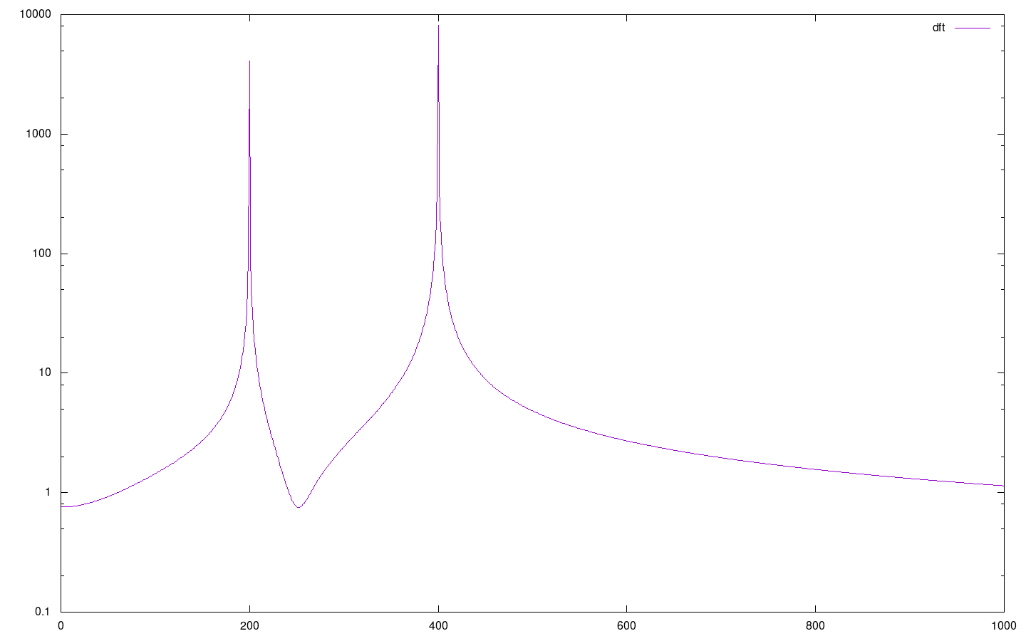 We can see the pikes at 200 and 400 that correspond to the sinuses in equation for x. Despite what one might expect - other values, although lower, are not zero. This is because we're trying to approximate something infinite using a finite set of discrete values. One can notice, that when the number of points we use is increased - the pikes het higher. In the limit, when going to ∞ points, we would get a Dirac-type distribution.
Sum of components cos(k·t) + i·sin(k·t) with weights being the values we got from the transformation approximates the input function f1, hence it is the answer to the first part of the task. What hasn't been mentioned yet is the fact, that for this the weights have to be complex numbers - and they are. In the dft plot above what is shown is not directly the set of values computed by fftw3 library, but rather their absolute values.
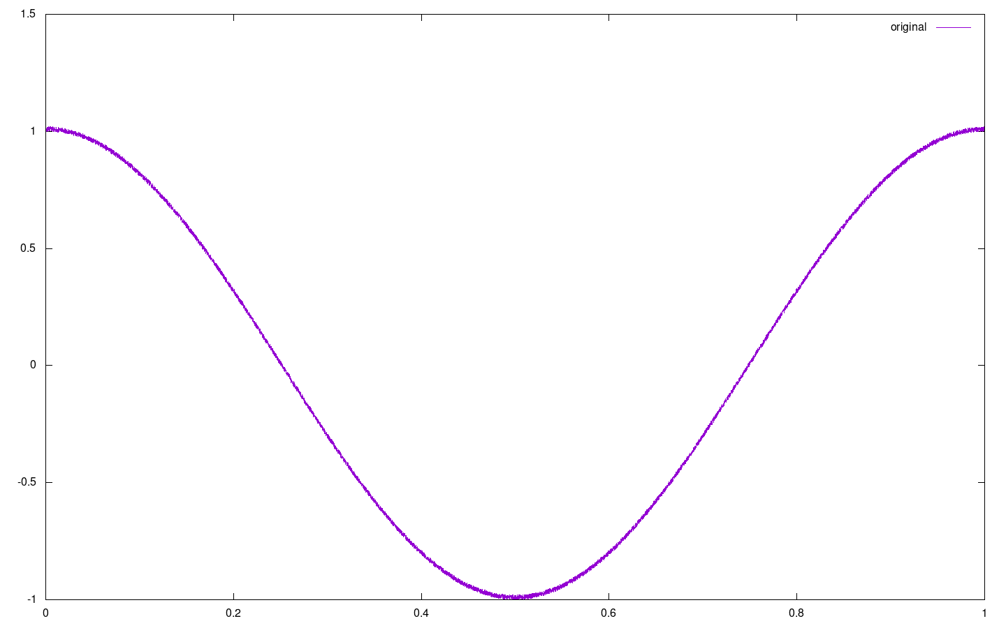
The second part of the task was to perform a dft of a cosinus function with some small random number (noise) added to each of it's values. The period of the cosinus was not specified, so x = cos(2·π·t) was assumed (represented by function f2 in the program) and pseudorandom values in the range [-0.01; 0.01] were taken. This is the plot of the original signal
 And the plot of it's dft (with x axis range of [0; 150] and logarithmic y scale)
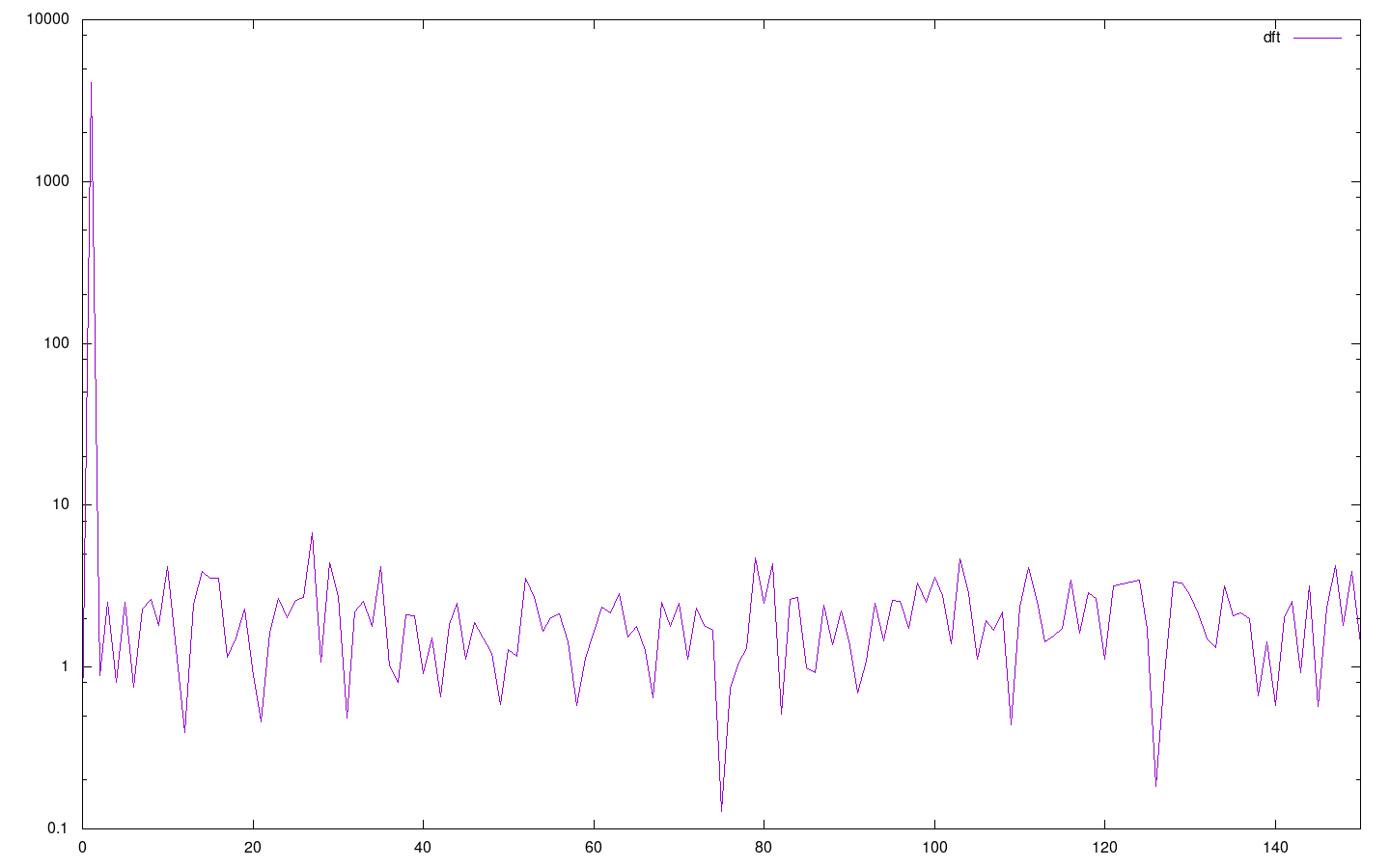 We can see, that there's a single pike at frequency 1 (corresponding to our main cosinus signal) and all other values are low and seemingly random.
The last part of the task was to remove all values of the dft with absolute value smaller than 50 and perform the inversed Fourier transform. This zeroed almost all of the 'random' part of the dft. Since the noise in the dft was the result of the noise in the original function, the result of the inversed Fourier transform was an almost perfect cosinus as can be seen below
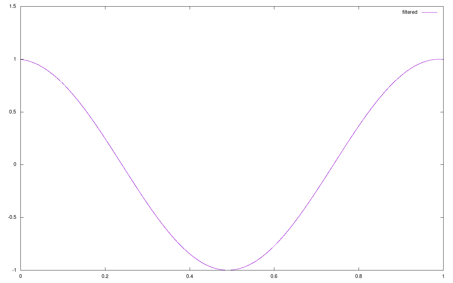 This worked, because the amplitude of the noise was small and so the amplitude of frequency components resulting from it was small (almost all absolute values of dft for frequencies other than 1 were smaller than 50). In case of stronger noise or a cap smaller than 50 this could possibly not work as well. Nevertheless, this (fast) Fourier transform example also presents one of the method used used for filtering periodical signals from noise. Other ways of filtering dft values also exist (e.g. convoluting with a predefined filter-function).